
Signal processing is a foundational discipline in electrical and computer engineering, enabling the analysis, interpretation, and manipulation of signals across various domains. One of the most important classifications of signals is based on periodicity. While periodic signals repeat over time, many real-world signals do not follow this behavior. These are known as non-periodic (aperiodic) signals.
This article provides a comprehensive and practical discussion of non-periodic signals, including their mathematical representation, properties, analysis techniques, and implementation using MATLAB. The content is structured to be beginner-friendly while still offering technical depth for advanced learners.
What is a Non-Periodic Signal?
A non-periodic signal is defined as a signal that does not repeat itself for any finite interval of time. In contrast to periodic signals, there is no fundamental period that satisfies the repetition condition.
Mathematical Definition:
This means there is no value of T for which the signal remains identical when shifted in time. Non-periodic signals often arise in natural and engineered systems where transient or time-varying behavior is observed.
Real-World Examples of Non-Periodic Signals
Non-periodic signals are extremely common in practical applications. Some typical examples include:
- Speech signals – human voice varies continuously and does not repeat exactly
- Transient signals – such as pulses or shocks in mechanical systems
- Exponential decay signals – seen in circuits and natural processes
- Random signals – noise in communication systems
Example of a simple non-periodic signal:
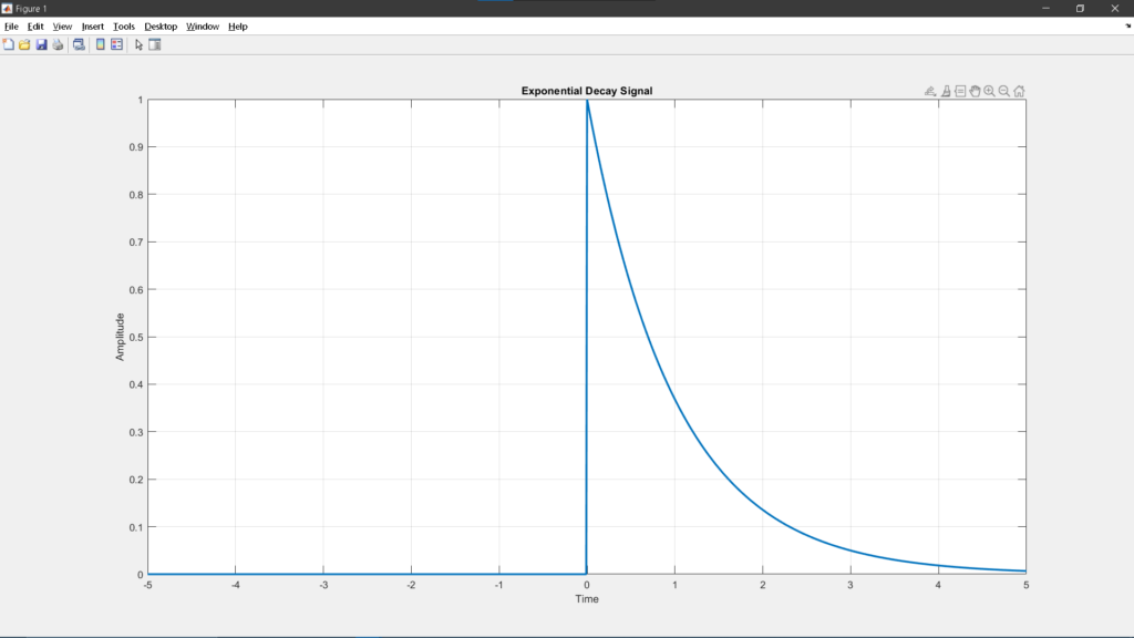
This signal decays over time and never repeats, making it a classic example of an aperiodic signal.
Energy and Power Classification
Signals are often categorized as either energy signals or power signals. Non-periodic signals typically fall under the category of energy signals.
Energy of a signal:
If the computed energy is finite, the signal is classified as an energy signal. Most non-periodic signals satisfy this condition.
In contrast, periodic signals generally have infinite energy but finite average power, making this distinction important for analysis.
Fourier Transform and Frequency Analysis
Since non-periodic signals do not repeat, the Fourier Series cannot be applied. Instead, we use the Fourier Transform, which converts a time-domain signal into its frequency-domain representation.
Fourier Transform Formula:
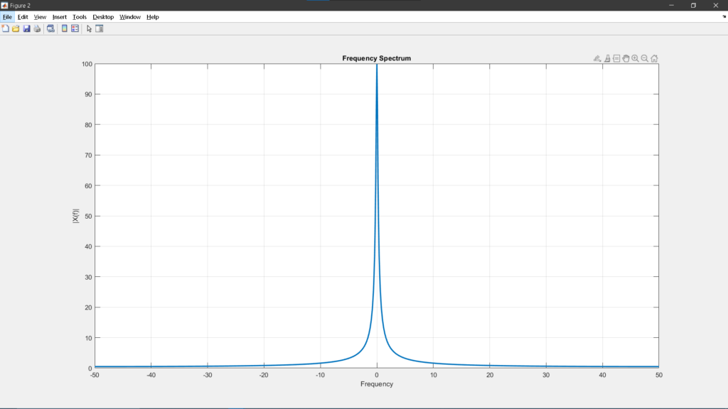
The result is a continuous frequency spectrum, allowing engineers to analyze how different frequency components contribute to the signal.
MATLAB Example 1: Exponential Decay Signal
This example demonstrates how to generate a non-periodic exponential decay signal and compute its Fourier Transform.
% Example 1: Exponential Decay Signal
clc; clear; close all;

t = -5:0.01:5;
a = 1;

% Define signal
x = exp(-a*t) .* (t >= 0);

% Plot time-domain signal
figure;
plot(t, x, 'LineWidth', 2);
grid on;
title('Exponential Decay Signal');
xlabel('Time');
ylabel('Amplitude');

% Compute FFT
X = fft(x);
f = linspace(-50, 50, length(X));
X_shifted = fftshift(X);

% Plot frequency spectrum
figure;
plot(f, abs(X_shifted), 'LineWidth', 2);
grid on;
title('Frequency Spectrum');
xlabel('Frequency');
ylabel('|X(f)|');
MATLAb Output #1:
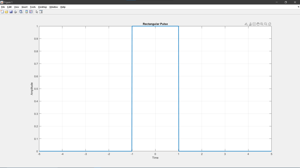
MATLAB Example 2: Rectangular Pulse Signal
A rectangular pulse is another classic example of a non-periodic signal. It is widely used in digital communications and system analysis.
Mathematical Representation:
% Example 2: Rectangular Pulse
clc; clear; close all;
t = -5:0.01:5;
T = 2;
% Define rectangular pulse
x = double(abs(t) <= T/2);
% Plot signal
figure;
plot(t, x, 'LineWidth', 2);
grid on;
title('Rectangular Pulse');
xlabel('Time');
ylabel('Amplitude');
% Fourier Transform
X = fft(x);
f = linspace(-50, 50, length(X));
X_shifted = fftshift(X);
% Plot spectrum
figure;
plot(f, abs(X_shifted), 'LineWidth', 2);
grid on;
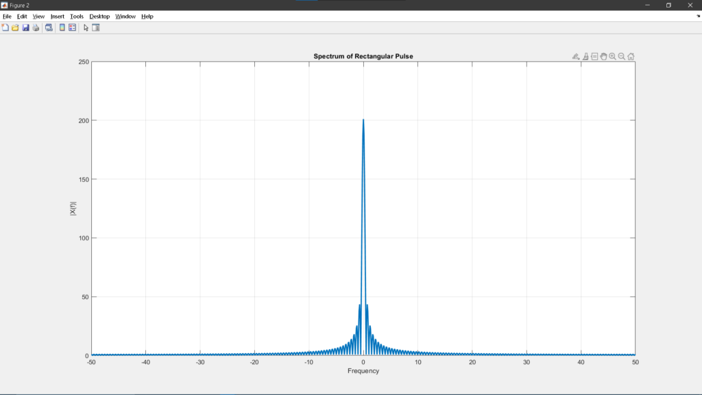
title('Spectrum of Rectangular Pulse');
xlabel('Frequency');
ylabel('|X(f)|');
MATLAB OUTPUT #2:
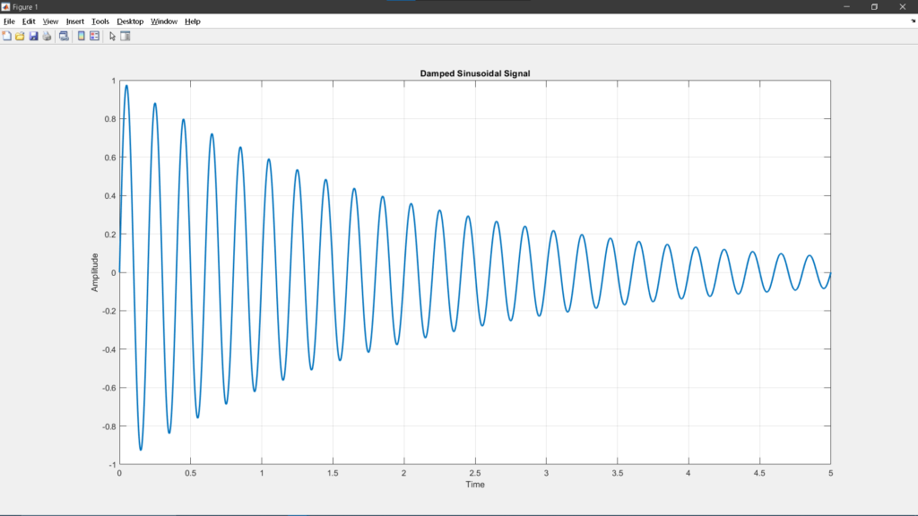
MATLAB Example 3: Damped Sinusoidal Signal
A damped sinusoid combines oscillatory and decaying behavior, making it a non-periodic signal commonly found in physical systems.
Mathematical Representation:
% Example 3: Damped Sinusoid
clc; clear; close all;
t = 0:0.001:5;
a = 0.5;
f0 = 5;
% Define signal
x = exp(-a*t) .* sin(2*pi*f0*t);
% Plot time-domain signal
figure;
plot(t, x, 'LineWidth', 2);
grid on;
title('Damped Sinusoidal Signal');
xlabel('Time');
ylabel('Amplitude');
% FFT
X = fft(x);
f = linspace(-50, 50, length(X));
X_shifted = fftshift(X);
% Plot frequency domain
figure;
plot(f, abs(X_shifted), 'LineWidth', 2);
grid on;
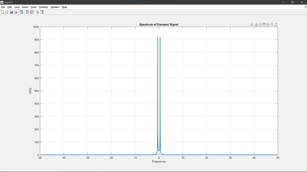
title('Spectrum of Damped Signal');
xlabel('Frequency');
ylabel('|X(f)|');
MATLAB OUTPUT #3:
Key Properties of Non-Periodic Signals
- No fundamental period
- Finite energy
- Continuous frequency spectrum
- Time-limited or transient behavior
These properties make non-periodic signals particularly useful in representing real-world systems where signals evolve over time without repetition.
Applications in Engineering
Non-periodic signals are widely used in various engineering disciplines:
- Communication Systems: Transient signals and pulses used in data transmission
- Biomedical Engineering: ECG and EEG signals are inherently non-periodic
- Control Systems: System responses to inputs are often non-repetitive
- Radar and Sonar: Pulse-based signal analysis
- Audio Processing: Speech and music signals
Why Non-Periodic Signals Matter
Understanding non-periodic signals is essential because most real-world signals are not perfectly periodic. Engineers must analyze signals that change over time, contain noise, or exist only for a short duration.
Tools such as the Fourier Transform and numerical simulation (e.g., MATLAB) provide powerful ways to study these signals in both time and frequency domains.
Guide Questions
- What defines a non-periodic signal, and how does it differ mathematically from a periodic signal?
- Why are most real-world signals considered non-periodic, and what are some practical examples in engineering applications?
- How is the energy of a non-periodic signal computed, and why are these signals typically classified as energy signals rather than power signals?
- Why is the Fourier Transform used instead of the Fourier Series for analyzing non-periodic signals?
- In the MATLAB examples provided, how does changing parameters (such as decay rate or frequency) affect the time-domain and frequency-domain representations of the signal?
- How does a rectangular pulse demonstrate non-periodic behavior, and what does its frequency spectrum reveal about signal bandwidth?
- What are the key characteristics that distinguish non-periodic signals in terms of repetition, energy, and spectral representation?
Conclusion
Non-periodic signals form a critical part of signal processing theory and applications. Unlike periodic signals, they do not repeat, making their analysis more complex but also more representative of real-world phenomena.
By understanding their mathematical foundations, energy characteristics, and frequency behavior, engineers can effectively analyze and process signals in a wide range of applications. MATLAB further enhances this understanding by allowing simulation and visualization of these signals in practical scenarios.
Mastering non-periodic signals equips you with the tools needed to tackle advanced topics in digital signal processing, communications, and system analysis.
Please answer the guide questions individually, this will serve as your activity for finals. Thank you and God bless everyone.
Agra, Elton Jhon B.
1.
A non-periodic signal doesn’t repeat in a fixed cycle. Mathematically, periodic signals use Fourier Series (discrete frequencies), while non-periodic ones use Fourier Transform (continuous spectrum).
2.
Most real-world signals don’t repeat perfectly—they’re finite or change unpredictably. Examples include speech audio, radar pulses, power system voltage spikes, and weather sensor data.
3.
Energy is calculated by integrating (or summing) the squared signal over all time. They’re called energy signals because total energy is finite, while average power is zero.
4.
Fourier Series only works for periodic signals. Fourier Transform is used for non-periodic ones to show their continuous range of frequencies.
5.
– Higher decay rate: Signal fades faster in time, spectrum narrows (less bandwidth).
– Higher frequency: Signal oscillates faster in time, spectrum shifts to higher frequencies.
6.
A rectangular pulse is finite and non-repeating. Its sinc-shaped spectrum shows bandwidth—narrower pulses mean wider bandwidths, and vice versa.
7.
– Repetition: No regular cycle.
– Energy: Finite total energy, zero average power.
– Spectrum: Continuous range (via Fourier Transform).
Energy- Finite
Spectral Representation- Continuous Spectrum
Ronald S. Florendo Jr.
1. Fundamental Characteristics
Non-periodic signals lack a repeating pattern. While periodic signals are analyzed using Fourier Series (yielding discrete frequency components), non-periodic signals require the Fourier Transform, which produces a continuous frequency spectrum.
2. Real-World Occurrences
Practical signals rarely exhibit perfect periodicity due to their finite duration or unpredictable nature. Common instances include vocal audio, radar transmissions, electrical transients in power networks, and meteorological sensor readings.
3. Energy Properties
Signal energy is determined through integration (for continuous signals) or summation (for discrete signals) of the squared amplitude across all time. These signals are termed energy signals because they contain limited total energy and consequently exhibit zero mean power.
4. Mathematical Tools
Fourier Series applies exclusively to periodic waveforms. For non-periodic analysis, the Fourier Transform reveals the complete continuous frequency distribution.
5. Spectral Relationships
– Temporal Decay: Rapid signal attenuation in time corresponds to reduced spectral spread (narrower bandwidth)
– Oscillation Rate: Increased temporal frequency shifts the spectral content toward higher frequency regions
6. Rectangular Pulse Illustration
A single rectangular pulse—finite in duration and non-repeating—demonstrates the inverse relationship between time and frequency domains through its sinc-function spectrum. Temporal compression (narrower pulse) necessitates spectral expansion (broader bandwidth), and conversely, temporal expansion permits spectral compression.
7. Defining Attributes
– Temporal Behavior: Absence of cyclic repetition
– Energy Profile: Bounded total energy with vanishing average power
– Frequency Representation:** Continuous spectral distribution via Fourier Transform